I do astrophotography. It’s the kind of hobby where you can’t afford to wing it: either I manage to squeeze the maximum out of the equipment and the conditions, or the night is lost. Reshooting quickly isn’t an option, because deep-sky exposure time is almost always measured in hours.
I usually shoot in color (OSC) and most often drive out to a spot to get the darkest sky possible. That’s why preparation starts long before I leave home. I need to pick a target and understand where it is in the sky right now, and whether it’s even worth going for it on this particular night. I need to assemble the setup for the task: mount the reducer, estimate exposure settings, configure the camera. And I need to make sure I don’t forget anything basic - cables, adapters, power - so that I don’t arrive on site only to find out I’m missing some tiny piece without which the whole system simply won’t start.
But hardware is only half the story. The other half is external factors. The weather forecast: cloud cover and its type, dust, temperature, wind, humidity. Seeing: atmospheric turbulence that directly hits sharpness, especially at longer focal lengths. A planetarium: the object’s track across the sky, its maximum altitude, the time of culmination, how many hours of usable exposure I can realistically collect in one outing, and how many more outings I’ll need. And of course the Moon, which can take the most valuable hours away so that, formally, “you can shoot,” but in practice the result will be mediocre. Plus the direction of light pollution from cities and settlements: the same object can sit on a dark background on one side of the sky and be hopelessly washed out on another.
All these parameters affect each other. There are many of them, they’re scattered across different tools, and it’s easy to make a mistake - I sometimes miss things myself. Sometimes the target turns out to be too low above the horizon and I have to re-aim the rig. Sometimes only on site do I realize the Moon hangs there until 2 a.m., which I simply forgot about, and I have to wait for it to set, otherwise the frame gets flooded with a flat gray background. It “works,” but it doesn’t deliver a consistent result.
At some point I started wondering: could I simplify the decision-making itself - whether to go shooting tonight or stay home. Do it in an Apple-like way: don’t try to cram dozens of parameters and icons onto the screen, don’t turn the process into an accountant’s simulator, but reduce it to one clear answer. Roughly: you see green, it means “you can go tonight.”
I built such a model. As the development language I chose Python, which already has a mature stack for astronomy as well as for working with time series and forecasts. I’m not a meteorologist, so I deliberately don’t build a physical model of the atmosphere. I evaluate a night the way a practicing astrophotographer evaluates it: through heuristics, compromises, and a subjective feel.
At the core of the planner is the hourly weather forecast from Open-Meteo. It’s one of the most convenient open sources: it provides consistent hourly data for most of the parameters I need and lets me look up to five days ahead. For practical astrophotography that’s almost always a sufficient horizon. Beyond that, forecast error grows so fast that any evaluation stops making sense. But even that wasn’t enough for me, so the model is supplemented with data from 7Timer. This service is geared toward astronomical tasks and provides additional indicators, including atmospheric transparency and seeing.
7Timer has an important limitation: its forecast time granularity is three hours. For visualizations and calculations that live in an hourly mode, that kind of data has to be extrapolated. Separately - about seeing. Formally, 7Timer provides it, but in practice this forecast is too smoothed and correlates poorly with what I actually see on the spot. Its point-based scale doesn’t translate well into clear values that can be compared against the resolving power of the equipment. So in the end I excluded 7Timer’s seeing forecast from the model and used indirect factors instead: winds aloft and the overall stability of the atmosphere.
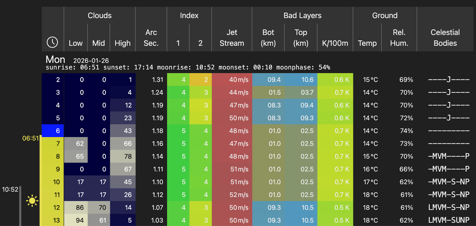
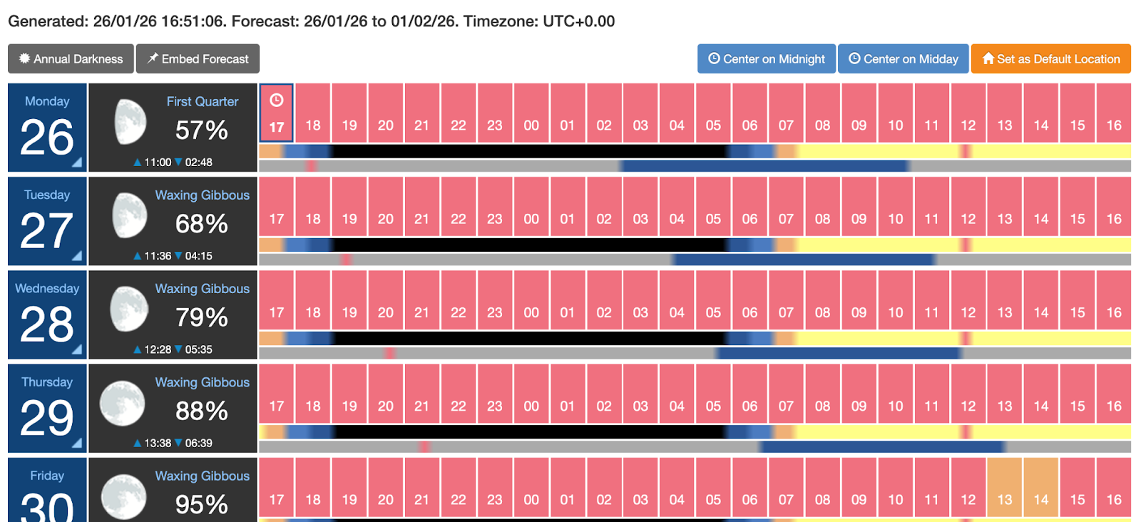
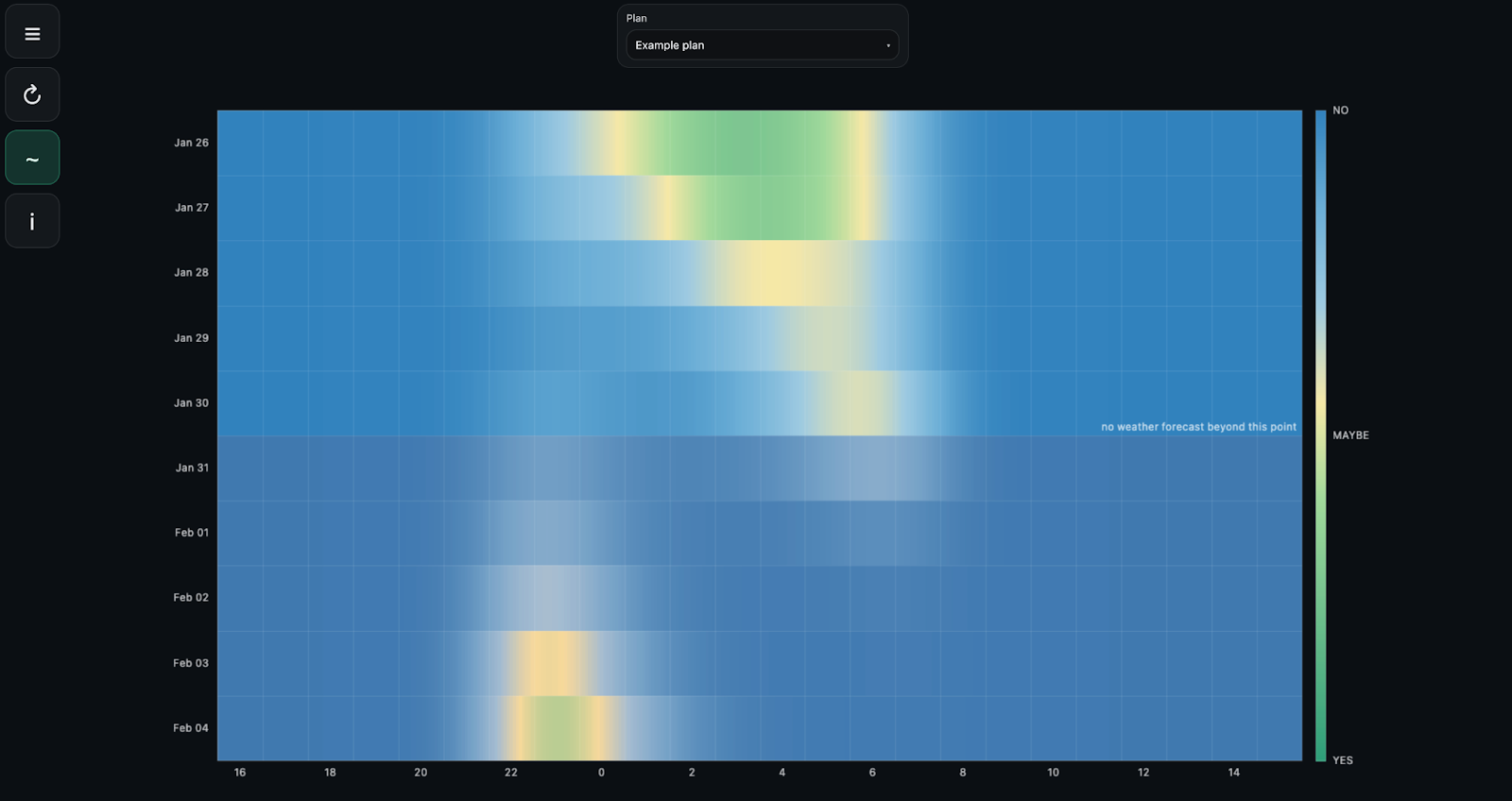
A five-day horizon isn’t enough to fill the screen with data completely, so the final heat map is split into two parts. The first is calculated with all weather factors and is limited by the forecast horizon. The second is built without weather and shows pure astronomical geometry: the motion of targets, the Moon, and the Sun. This lets me see “windows of opportunity” in advance, even if the specific conditions will only become clear closer to the date.
Experienced astrophotographers will reasonably say: “why do all this if Clear Outside or Meteoblue exist?” Because in my model I went further. First, I account for the parameters of the setup that will be used for the shoot, and the object’s position. Second, I remove informational noise: instead of columns of data, conditional icons, and various scales, there is a single heat map in “date - hour - quality” coordinates. The decision is made literally at a glance, without having to keep in mind what “two humidity droplets” mean and how critical “three wind lines” are.
Once I had settled on the meteorological data sources and the astronomical calculations, I needed to solve one more mundane issue: object identification. The same object can have different names in different catalogs, and manually looking up coordinates quickly turns into an annoying routine. To remove that, the SIMBAD catalog is used for name resolution: the user enters a familiar name, and the system converts it into precise coordinates. To compute the motion of the Moon and the Sun and their altitude above the horizon, I use Astropy - a standard tool in the astronomical Python stack that provides sufficient accuracy for my purposes.
Raw forecast data in its original form is poorly suited for direct use. Parameters are measured on different scales, have different “directions,” and are interpreted differently: sometimes higher is better, sometimes it’s the opposite; sometimes the effect is linear, sometimes it’s threshold-based or clearly non-linear. That’s why bringing everything to a single semantics is the first mandatory step. I flip the scales so that they all point in one direction, and then normalize the values into a 0 to 1 range. Essentially it’s a penalty scale: 0 means the most favorable conditions for that parameter, 1 means clearly bad. After that the parameters become comparable: they can be combined, weighted, and aggregated without losing intuitive meaning.
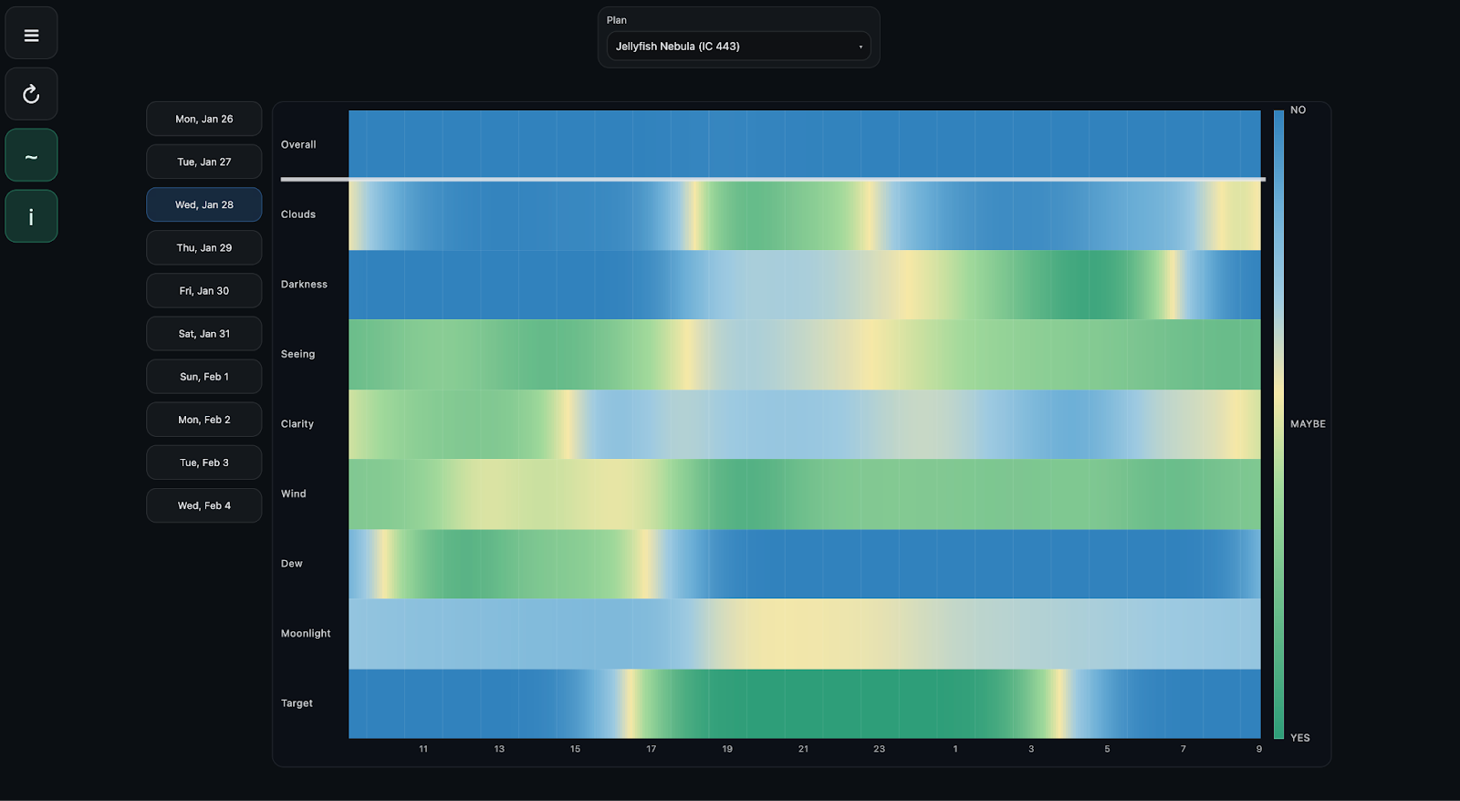
At the same stage, integrated metrics are formed, each responsible for a separate aspect of an imaging night. In the current version of the model these are cloud cover, “sky darkness” without anthropogenic light pollution, the Moon’s position and phase, seeing, atmospheric transparency, wind, humidity, and the target’s position.
Cloud cover
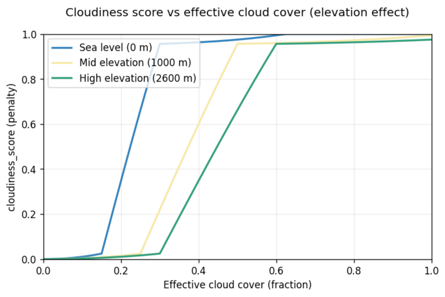
Cloud cover is the most obvious and at the same time the most treacherous factor. At first glance the logic is binary: there are clouds - you can’t shoot; there are no clouds - you can. In reality it’s more complicated. Different cloud layers affect things differently, and partial cloudiness often turns out to be no better than a uniformly overcast sky.
The input data comes from Open-Meteo and arrives as three independent values: low, mid, and high cloud cover in percent. I fold them into an effective cloud fraction using weights. The idea is simple: low dense clouds are almost always fatal; high clouds sometimes only eat contrast and transparency; mid-level clouds sit in between.
Separately, I add a heuristic for the altitude of the shooting location, based on a practical observation: if I’m above the inversion layer, I do in fact more often end up above the clouds that look scary in the forecast. For high-altitude locations, the influence of low and partially mid-level clouds is reduced.
Sky darkness
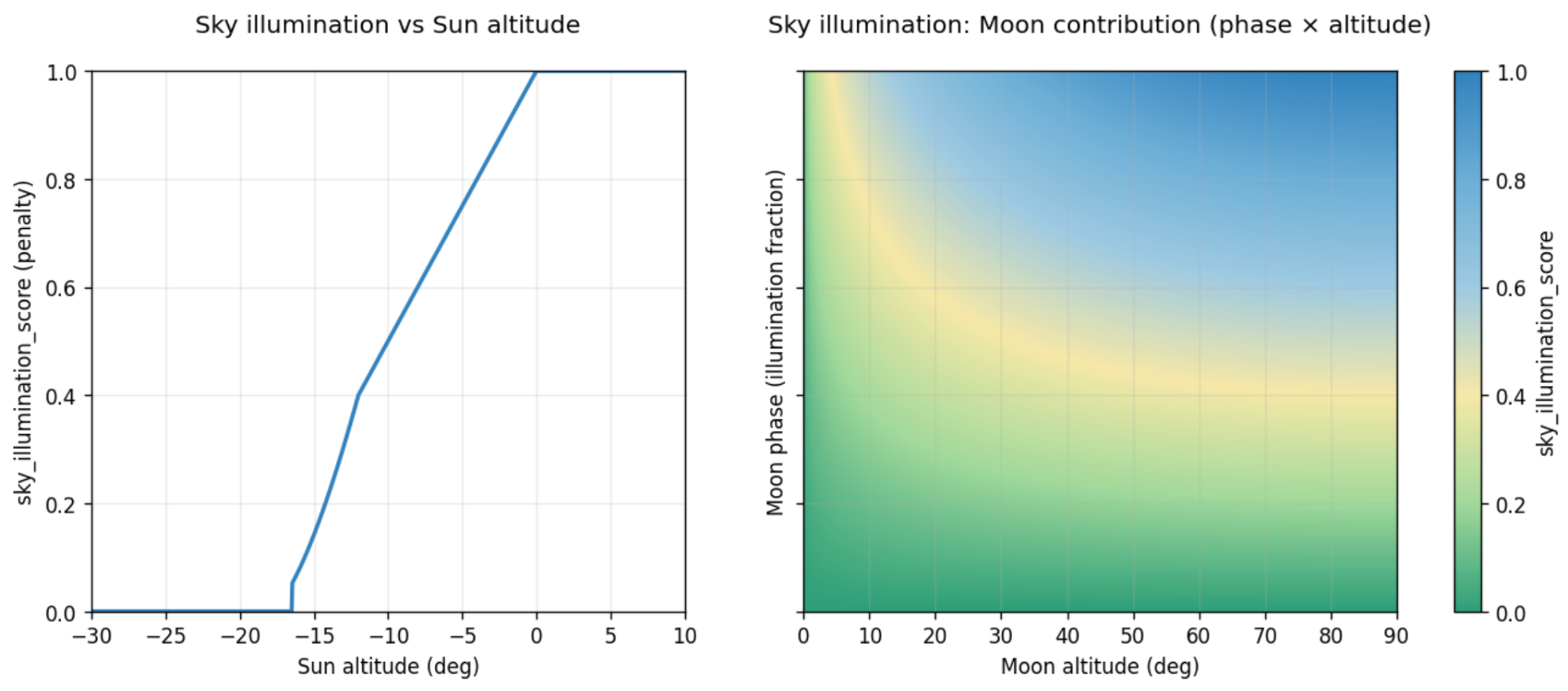
Even under a perfectly clear sky, shooting can be completely pointless if the background is too bright. The sky-darkness metric is computed from astronomical geometry and depends on the positions of the Sun and the Moon; it does not account for anthropogenic light pollution. The more the Sun or Moon illuminates the sky, the worse this metric becomes.
First, the Sun’s contribution is computed. While it is deep enough below the horizon, its contribution is zero. As it rises, the twilight zone begins, where the sky brightens quickly. This transition is defined by a power curve: that’s how I control how sharply twilight conditions move into the “bad” category. After that, the metric quickly goes to its maximum value - under daylight, deep-sky astrophotography is obviously impossible.
Separately, the Moon’s contribution is computed - its brightness is estimated as proportional to its phase and its altitude above the horizon. The phase is given by the illuminated fraction of the disk, and altitude is taken through the sine of the angle: a low Moon affects the background much less than the same phase high in the sky. If the Moon is below the horizon, its contribution is zero.
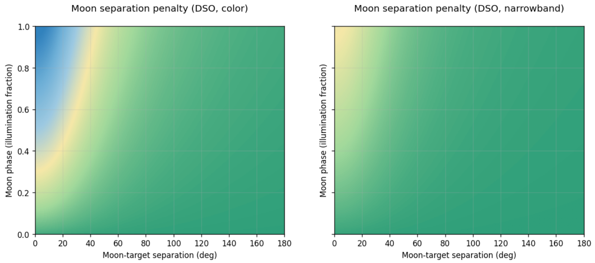
Angular distance to the Moon
This metric is defined by the Moon’s phase, the angular distance between the Moon and the target, and the sensitivity of a particular imaging scenario to moonlight (OSC or narrowband). Phase is handled non-linearly and is never fully zeroed out: even a thin crescent can spoil the background if it’s close to the target. Angular distance works as a decaying function. When the Moon is close to the object, the score is close to its maximum. As the distance increases, the influence drops quickly. That is exactly what is observed in practice: under a bright Moon you can still shoot if the object is far from it in the sky, even though the overall sky background rises and contrast falls.
Additionally, there is a strength coefficient that depends on the type of target and the equipment. For deep-sky targets, the penalty is maximal, but it is deliberately reduced for narrowband imaging, where the contribution of scattered moonlight is noticeably smaller.
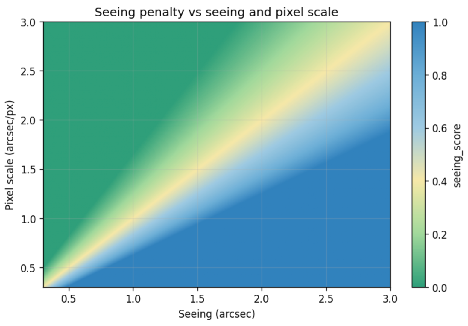
Seeing
Seeing should not be treated as an absolute property of the night in the sense of “low is good, high is bad.” In practice it only makes sense in combination with specific equipment that determines the imaging scale.
This score is built from an estimate of atmospheric stability in arcseconds, computed from winds in the upper layers of the atmosphere (the jet stream), and from the equipment’s pixel scale in arcseconds per pixel.
I’m not trying to guess what value is globally good or bad. If atmospheric blur is smaller than or comparable to the pixel size, the atmosphere does not limit the result. If the blur is several times larger than the pixel scale, further increasing resolution is pointless - the signal will be blurred anyway.
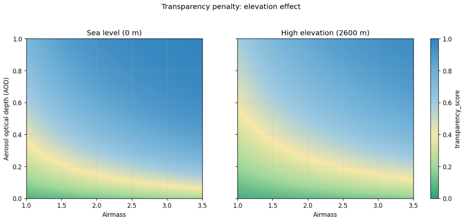
Atmospheric transparency
Atmospheric transparency determines how much useful signal from the target reaches the camera at all. Unlike seeing, which hits detail, transparency affects contrast and depth: how quickly faint structures drown in the background.
The estimate is based on an approximate model of atmospheric transmission along the line of sight to the target. The key parameter is the target’s airmass: the lower the target is above the horizon, the thicker the layer of atmosphere the light passes through, and the more losses accumulate. That is why low targets are penalized harshly.
The base optical thickness consists of two components. The first is molecular scattering in the air, which decreases with the altitude of the shooting location: up in the mountains the atmosphere is literally thinner. This is modeled as an exponential attenuation of vertical optical thickness. The second component is aerosols, approximated via the forecast aerosol optical depth.
On top of optical thickness, two additional multiplicative factors are applied. The first is dust: airborne dust is accounted for by a separate coefficient that affects transmission attenuation as particle concentration increases. The second is humidity. High relative humidity by itself does not yet mean poor transparency; if you penalize it directly, it’s easy to get false “bad” scores. So the humidity contribution is turned on gradually and is strengthened only when there are signs of real fog or dew formation, or when humidity is extremely high. Otherwise the impact is reduced.
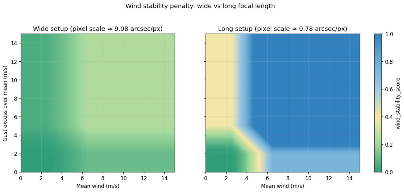
Wind stability
Wind affects imaging in several ways. The problem is not only the average speed, but how it is transmitted through a specific mechanical system - tube, mount, tripod - and how it manifests at a particular imaging scale.
The inputs are the forecast wind speed and gusts at 10 meters, as well as equipment parameters from which pixel scale is computed. This is crucial: the same wind feels different on a short focal length setup and on a long tube with small pixels. I deliberately do not try to account for the setup’s wind sail area - this parameter is too hard to define and include correctly in the model.
The calculation starts by isolating “excess” wind. Up to a certain threshold, wind is considered conditionally safe: it either does not transmit into the system or is easily compensated by guiding. Everything above the threshold is treated as a source of instability. Gusts are handled not as an absolute value, but as an excess over the mean wind: sharp changes are what most often knock the system out of balance. A steady wind is often tolerated better than a gusty one, and this is reflected in the score logic.
Then the key part kicks in: scaling by imaging sensitivity. The smaller the pixel scale, the higher the sensitivity to the same mechanical oscillations. This is captured by a coefficient that increases the penalty for high-resolution setups and reduces it for wide-field ones.
This score complements seeing well: one describes atmospheric instability, the other mechanical instability. Together they answer the practical question: will the system be able to hold the star where it should be throughout the exposure.
Dew risk
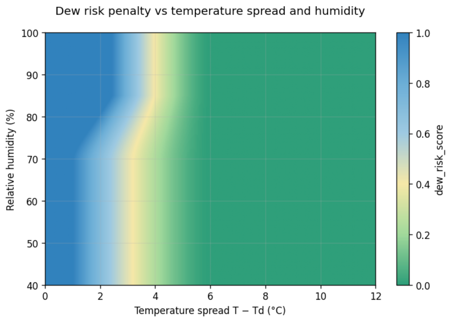
Dew and fogging of optics is one of the most unpleasant ways to lose hours of exposure. I already included humidity in the atmospheric transparency estimate as degraded transparency; here I only evaluate the risk of condensation on the optics.
The main driver of the model is the difference between air temperature and dew point. That is what determines how close the system is to condensation. If the difference is large, the risk is minimal almost regardless of other factors. If the temperature is close to the dew point, the situation becomes dangerous even at moderate humidity. So the temperature spread is the primary factor, and the rest only strengthens or weakens the final score.
Relative humidity is used as an amplifier. Above a safe level, the penalty starts to grow and rises especially quickly as it approaches critical values. Ventilation is also considered: wind reduces the likelihood of dew through heat exchange. This effect is applied only after a minimum wind speed threshold and has limited strength: it can noticeably reduce the risk but cannot eliminate it completely. A soft correction for the altitude of the shooting location is also added: at high sites, dew forms less often on average than in lowlands, so the final penalty is slightly reduced.
In the integral rating, this score has intentionally low weight. In real practice, the dew problem is often solved technically - with heaters, dew shields, and covers. So high dew risk is not a stop factor, but a useful warning.
Target observability
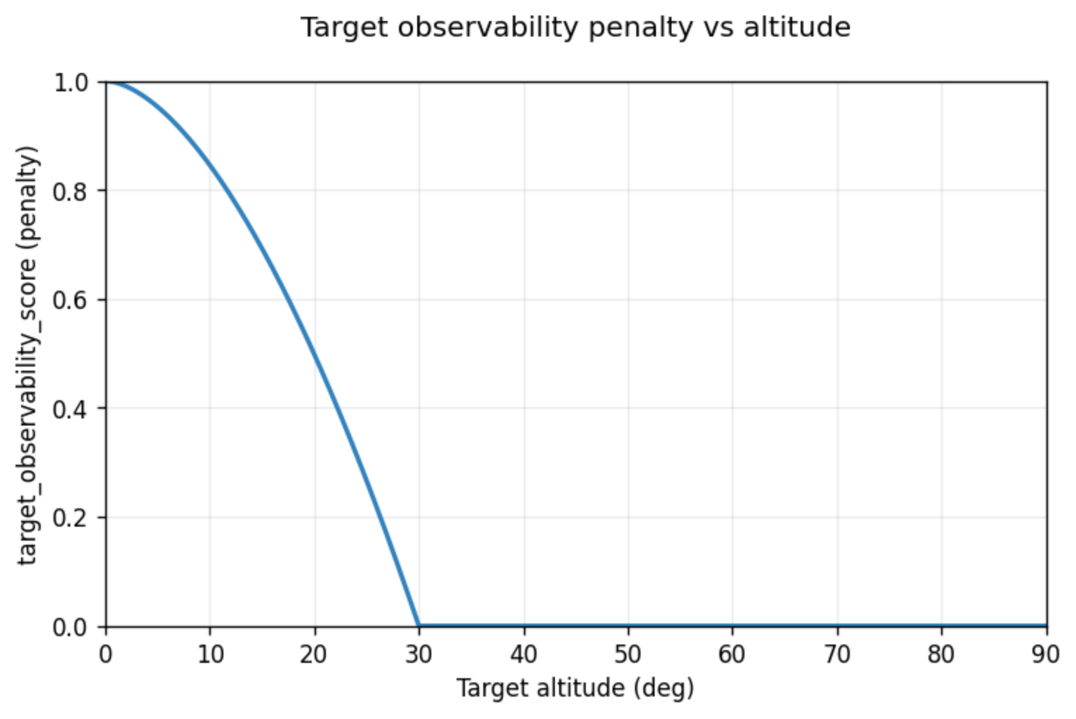
Regardless of weather and darkness, there is a basic geometric constraint: the target must be above the horizon and at a reasonable altitude. If this condition is not met, the other metrics lose their meaning. That is why the model has a separate observability score.
The input is the target altitude above the horizon, computed by the astronomical pipeline. If the target is below the horizon, the score is rigidly equal to one: this is not merely “hard to see,” it is a complete absence of observing conditions. If the target is above a defined comfortable altitude (30 degrees), the parameter’s contribution is zero: geometric constraints are considered lifted, and then atmosphere, the Moon, and mechanics take over. Between the horizon and the comfortable altitude, a smooth non-linear transition is used: the closer to the horizon, the stronger the penalty, which matches the real feeling - even if the target is formally “above the horizon,” it can be blocked by terrain, low contrast, or blurred.
Integral night rating
All the previous scores exist for one purpose: to collapse them into a final rating that can be visualized and used for decisions. The result is built as an integral assessment of sky quality for each hour of the day.
I deliberately split the integral model into two levels: hard blockers (gates) and soft quality factors. To combine scores I use a weighted noisy-OR that neatly merges independent risks: each factor reduces the chance of a “good hour,” and those chances are multiplied. A mean works poorly here: one catastrophic factor is easily “smeared out” by several good ones. A minimum is too strict and does not reflect gradual degradation well.
The gate model answers whether it makes sense to consider an hour as potentially usable at all. It includes factors that can kill imaging almost on their own: darkness, cloud cover, and the fact that the target is below the horizon. These channels are aggregated via weighted noisy-OR so that if one factor is clearly bad, the result quickly becomes bad regardless of the others. At the same time the logic remains continuous: it’s not a binary if, but a smooth yet strict function. Gate metrics dominate the final rating: if one of them is close to one, the integral score will also be close to one, even if everything else is perfect. This is how the model protects itself from false positives - for example, when seeing is excellent but the sky is in twilight.
If the basic conditions are formally acceptable, the quality model turns on. It answers how large the risks are of ruining the data if I shoot during that hour. All the remaining metrics are taken into account here.
Cloud cover is a special case. It appears on both levels for a reason: in the gate it answers “can I shoot at all,” and in quality it describes degradation under partial or high cloud, when shooting is still formally possible but the result is already getting worse and halos appear around stars. Before aggregation, some channels go through non-linear “shaping” to change sensitivity in the middle range: some parameters are penalized gently for small deviations but sharply as they worsen. This matters for scores where “almost bad” often feels worse than the numbers suggest, and it helps bring the result closer to human perception.
As a result, I get a picture that a human can read without decoding. I open the heat map and in a second I understand what used to take tens of minutes.
I’ve been using this tool for a couple of months now, and so far all noticeable mismatches with reality come down to one reason: the weather forecast itself is wrong. In that sense the model behaves honestly: it doesn’t create an illusion of precision, it just neatly folds the available data into a clear form. If the forecast updates, I refresh the data, and the picture becomes clear again.
The only thing I’m missing right now for a complete picture is accounting for anthropogenic light pollution. And here I deliberately do not intend to go down the path of an “ideal” model with terrain, shielding, and attempts to compute absolute sky brightness: such systems quickly become cumbersome and start lying confidently where the data simply doesn’t exist. Instead, I want to add exactly what is useful in practice: compute the azimuth to the target by hour, determine the presence of bright sources in that direction, and add the overall sky background at the shooting site as a correction factor.
At this point I have a simple working tool that genuinely helps me make decisions. If you want to see what it looks like, it’s available here: https://sky.lonely-lockley.ru